Attention
4 minute read
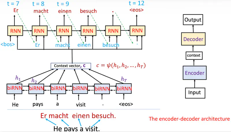
Entire input (\(h_1, h_2, \dots, h_T\) ) is encoded into one fixed-length vector.
So, as the length of an input sentence increases performance of a basic encoder–decoder deteriorates rapidly,
because of vanishing gradient problem.
Read more about Vanishing Gradient Problem
Encoder-Decoder Architecture (RNN)
Decoder decides parts of the source sentence to pay attention to.
By letting the decoder have an attention mechanism, we relieve the encoder from the burden of having to
encode all information in the source sentence into a fixed-length vector.
While decoding an output pay attention to only relevant inputs.
Decoder Context
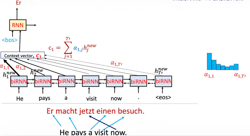
Note: Now the decoder context is not fixed.
While predicting the next word, the decoder (instead of relying only on the final encoder hidden state)
dynamically pays attention to only relevant context from encoder at that time step.
Why it matters?
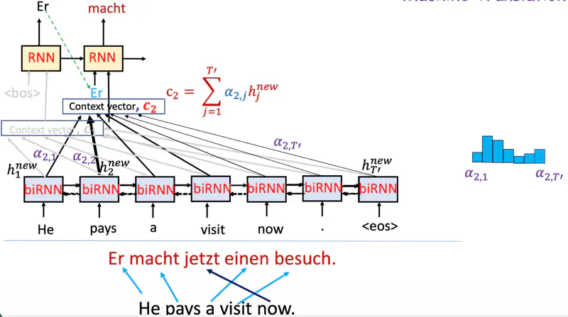
This allows the decoder to “look back” at the entire input sequence, preventing the information loss that occurs
in basic encoder-decoder models when handling long sentences.
Goal
To determine the context vector (relevant) at each time step of decoder.
Before that we need to understand the meaning of few terms, viz., “Query”, “Key” & “Value”.
Research Paper: Neural Machine Translation by Jointly Learning to Align and Translate ; Dzmitry Bahdanau, Kyunghyun Cho, Yoshua Bengio, 2014, https://arxiv.org/pdf/1409.0473
In the context of Attention mechanism, Query (Q), Key (K), and Value (V) are metaphors borrowed from retrieval systems
(like a database or a search engine) to describe how information is accessed.
Let’s understand these terms via a “data fitting” problem.
Data Fitting
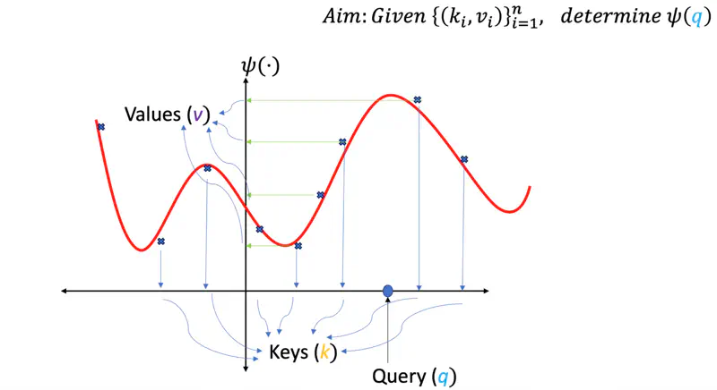
We are give some data points, i.e, some keys (\(k_i\)) and corresponding values (\(v_i\)), and the task is to find
the best fit curve (\(\psi(q)\)) so that in future if we have a new query point ‘\(q\)’ we should be able
to determine(predict) the corresponding value for the query point.
Something similar to linear regression.
Similarity Score
One of the ways can be that we find the similarity (dot product) of the query point ‘\(q\)’ with every key (\(k_i\)),
if the similarity score is high means they are closer, and vice versa, then we can take the corresponding values (\(v_i\))
scaled by the similarity score and sum them up to get the predicted value for the query point ‘\(q\)’.
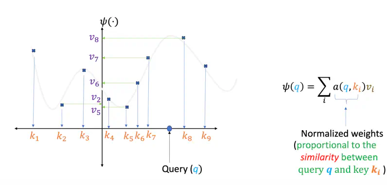
Here, in above example query point ‘\(q\)’ is closer to keys \(k_7\) and \(k_8\), hence the predicted value for the query will be more close to \(v_7\) and \(v_8\) as compared to \(v_1\) or \(v_2\), which are quite far away.
Softmax
Moreover, we can apply a softmax on the similarity scores, so that the higher scores are amplified (winner takes most),
thus giving us better prediction.
This turns our prediction into a weighted average of the values \(v_i\).
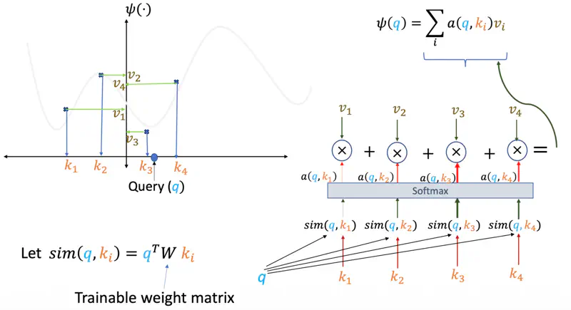
Note: Instead of a fixed curve, the model learns the best way to represent ‘\(q\)’ and ‘\(k\)’
so that the “similarity” perfectly captures the relationship we re trying to predict.
We can also have a trainable weight matrix ‘\(W\)’ whose parameters can be learnt during training.
Attention
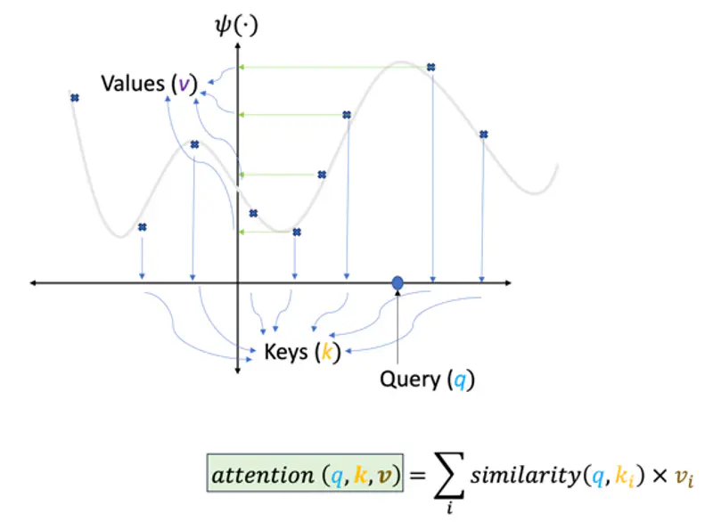
Therefore, the attention score (\(q,k,v\)) for a query ‘\(q\)’, given keys ‘\(k_i\)’ and values ‘\(v_i\)’ is the summation of all query and key similarity scores similarity(\(q, k_i\)) multiplied by their corresponding values ‘\(v_i\)’.
Bahdanau Attention was designed for the RNN based encoder-decoder architecture used for machine translation.
Encoder Decoder (Cross) Attention
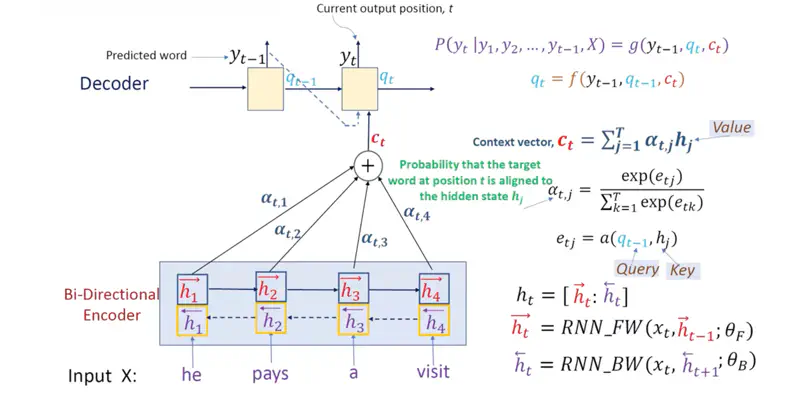
- Query: Decoder’s previous state (\(q_{t-1}\)).
- Keys: Encoder’s knowledge points from the source sentence, i.e, hidden state (\(h_j\)).
- Values: Encoder’s knowledge points from the source sentence, i.e, hidden state (\(h_j\)).
- The model “fits” the current context by calculating which source points are most relevant to the word it is currently predicting.
Let us understand all the terminologies used in the diagram above in detail:
- Alignment Function: A small neural network to see how well the Decoder’s “need” matches the Encoder’s “offer”.
- \(a(q_{t−1}, h_j) = v_a^T \tanh(W_a q_{t-1} + U_a h_j)\); Additive Attention
- Alignment Score or Energy, \(e_{tj} = a(q_{t−1}, h_j)\)
- Attention Weight: Softmax operation ; takes the raw “importance scores” (\(e_{ij}\)) and converts them into a probability distribution.
- Ensures that all \(\alpha_{ij}\)are between 0 and 1 and that they sum to 1.
- This makes the context vector (\(c_t\)) a stable weighted average.
- Softmax, \(\alpha_{tj} = \frac{\exp(e_{tj})}{\sum_{k=1}^T \exp(e_{tk})}\)
- Context Vector: Weighted sum of the encoder hidden states (the Values).
- \(c_t = \sum_{j=1}^T \alpha_{tj} h_j\)
Note: Bahdanau used additive attention, which is slow because of the addition step.
Dot Product Attention
\[a(q_{t−1}, h_j) = q_{t-1} ^T h_j\]Note: Faster to compute dot product than additive attention.
Research Paper: Effective Approaches to Attention-based Neural Machine Translation, Luong et al., 2015, https://arxiv.org/pdf/1508.04025
Scaled Dot Product Attention
\[a(q_{t−1}, h_j) = \frac{q_{t-1} ^T h_j}{\sqrt{dim(h_j)}}\]Research Paper: Attention Is All You Need, Vaswani et al. , 2017, https://arxiv.org/pdf/1706.03762